Scanner Devices
The scanner device is used to control a set of galvometric mirrors to precisely direct a scanning laser beam. The device allows the user to specify the desired laser spot location by graphically selecting the location from within a camera module. The transformation between camera coordinates and X,Y voltages is determined by an automatic calibration procedure.
Configuration
Example scanner configuration:
Scanner:
    driver: 'Scanner'
    parentDevice: 'Microscope'       ## Scanner is rigidly connected to scope, inherits its transformations.
    calibrationDir: 'config\\ScannerCalibration'
    XAxis:
        device: 'DAQ'
        channel: '/Dev1/ao2'
        type: 'ao'
    YAxis:
        device: 'DAQ'
        channel: '/Dev1/ao3'
        type: 'ao'
    defaultCamera: "Camera"
    defaultLaser: "Laser-UV"
    commandLimits: -3, 3
    #offVoltage: 0, -3    ## "off" position when simulating a virtual shutter
    #shutterLasers: ['Laser-UV']  ## list of lasers for which we should simulate a shutter by default
Manager Interface
Calibration
The primary function of the Scanner device is to allow the user to select the laser spot position relative to camera coordinates. The scanner device, therefore, must know the corresponding transformation. This is achieved through an automatic calibration routine:
The pre-stored camera configuration is loaded
The camera begins recording at a high frame rate (30-100fps)
The mirror voltages are systematically varied to raster-scan the laser spot
Spots are automatically detected in each camera frame and matched with their corresponding voltages
The relationship between camera coordinates and mirror voltages is determined by linear regression
The camera is returned to its previous state
If there are multiple cameras, lasers, or objective lenses, one calibration must be made for each combination. This process is somewhat complex and requires that the user ensure the hardware is configured properly prior to calibration:
The camera must indicate its frame exposure times via a TTL signal connected to the DAQ board.
The camera must be acquiring at a high frame rate, usually 30fps or more. If the camera is acquiring too slowly, then too few spots will be captured to make an accurate linear regression.
The exposure time of each frame must be short, usually less than 5ms. Otherwise, the spot images captured will be ‘smeared’ and their location will not be detected accurately.
The laser spot must be brightly visible to the camera
Objective lenses must be clean
Laser spot should be projected on a flat, bright surface (we recommend using small pieces of fluorescent tape or plastic)
To achieve these requirements, it is common to configure the camera to use binning and to operate over a restricted region of interest. When the camera is configured with all appropriate settings, click the “Store Camera Config” button in the manager interface. All calibrations from then on will load these camera settings before starting and restore the original settings afterward.
When all hardware is configured correctly, do the following to start a calibration:
Select the laser and camera to be calibrated in the manager interface
Be sure that the correct microscope objective is selected in the microscope interface
Click ‘Calibrate’.
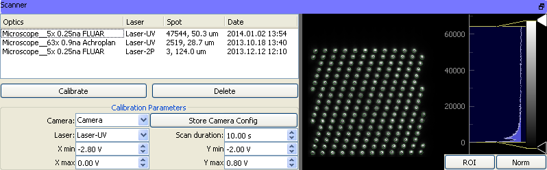
The results of the calibration should appear in the window to the right. There should be clear laser spots with circles drawn around them. In the table, the Spot column lists a relative measure of the amount of light in the spot, and diameter of the spot where intensity drops off to 1/e. This diameter also determines the size of the targets used to setup and run protocols.
Calibrations are stored for each combination of camera/objective/laser. When you calibrate, any calibrations previously stored for the combination you’re calibrating are overwritten.
Calibration Parameters
Laser and Camera selection boxes: You can tell the scanner which camera and laser to use (if you have more than one) for the calibration by selecting them here.
Scan Duration: Sets the total amount of time for the calibration. For cameras that are slow or not sensitive enough, increase the scan duration to allow more time for frame collection and integration. If you run into memory errors, decrease the scan duration, or increase the binning on the camera. (Remember to re-store the camera settings if you increase the binning by clicking the “Store Camera Config” button.)
X & Y Min and Max: Set the range of voltages that are scanned over during the calibration.
Store Camera Config: Clicking this button stores the current configuration of the camera to use for future calibrations. If you are having trouble calibrating, it is a good idea to manually adjust all the camera settings and then re-click “Store Camera Config.”
Virtual Shutter
The scanner can be used to simulate a shutter by directing the laser to a beam block outside the microscope illumination path. If you use this make sure that when in the “off” position the laser is directed onto an absorbant surface (please use common sense). The ‘off’ position can be set in the calibration file using the ‘offVoltage’ key.
Task Runner Interface
To include the scanner in a protocol, first mark the Scanner check box in the list of devices. This should bring up the Scanner’s protocol interface.
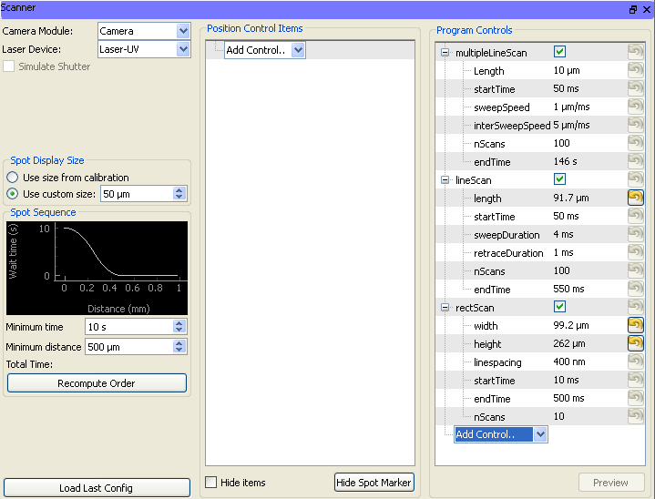
Controls
Camera and Laser: Select the camera and laser that you want to use in the protocol. Be sure that you have calibrated whatever combination of camera and laser that you choose.
Simulate Shutter Check: This determines whether you are using the Virtual Shutter function or not. If checked, the scanner will send the spot to the “off” position whenever the shutter is closed (set this in the scanner configuration using the ‘offVoltage’ key.) If not checked, the scanner ignores the virtual shutter option and you need to have a real shutter somewhere in the path.
Spot Size Display: This determines the size that is used to display stimulation spots. By default the size from the calibration is used, but the user can also adjust the spot display size by selecting “Use custom display size” and setting the size accordingly. This option can be useful if the user wants to space stimulation spots at a high density.
Minimum Time and Minimum Distance: These two numbers determine how frequently sites can be stimulated in space and time. If Minimum Time is 5 seconds and Minimum Distance is 500 microns, this means that when Spot A is stimulated, spots that are less then 500 microns will have a delay to be stimulated. The delay time for spots at each specific distance is shown in the plot above these controls. Spots further than the Minimum Distance away can be stimulated with no delay.
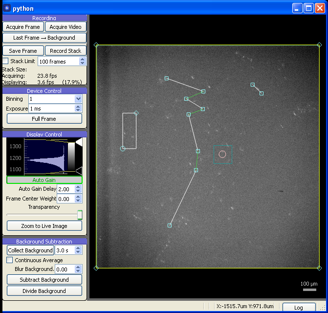
Adding Targets
For sequences of scans there is currently only one type of target implemented: A spot. You can add target spots individually, or you can add them as grids. Eventually, we will implement more complex scanning patterns that will include scanning along lines (including spirals), and stimulating multiple locations within the same trace. Some of this is implemented in the Scan Programs section (below), but we intend to add a mechanism for sequencing a specific scan pattern (say a spiral) over a series of locations…
Whenever there is a scanner protocol interface open, a pink target spot will appear in the selected camera. This pink spot is a test spot and will be stimulated whenever Test Single or Record Single is clicked.
To add targets that will be stimulated in sequence click on the “Add Control…” box in the Position Control Items box and select the item you want to add. Adding a Grid will add a grid of points to the camera window. You can adjust the position of this grid in the camera window. To translate the grid click in the middle of the grid and drag. To rotate the grid, click and drag on of the circular handles on the corner of the grid. And to scale the grid, click and drag one of the square handles. Grids also have adjustable features:
Layout: Options are ‘Hexagonal’ and ‘Square’. This determines whether the grid is laid out in a hexagonal or square packing pattern.
Spacing: This controls the spacing of the stimulation spots. This has no effect on the size of the stimulation spot!
You can also add a Point, which will add a single stimulation point to the protocol. This point will appear as a circle in the selected camera module, and can be dragged to adjust its position.
You can add as many grids and points to a protocol sequence as you like. If you do not want to use a grid or point during a particular protocol sequence, you can either uncheck it in the Position Control Items list (so that it will be available in the future), or you can delete it by right-clicking it in the Position Control Items list and choosing Remove.
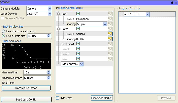
Active target points will appear in white by default.
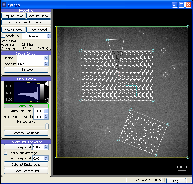
If you want a grid (perhaps over the area around a cell) but have an area that you don’t want to stimulate (for example where an electrode is over the slice) you can add an Occlusion. You can adjust the location of the corners of the occlusion by dragging any of the corner handles, and you can translate the occlusion by clicking and dragging it by the middle. Any points whose centers fall within the occlusion will be removed from the target list (and appear in dark grey in the camera window).