Plots and interactive views

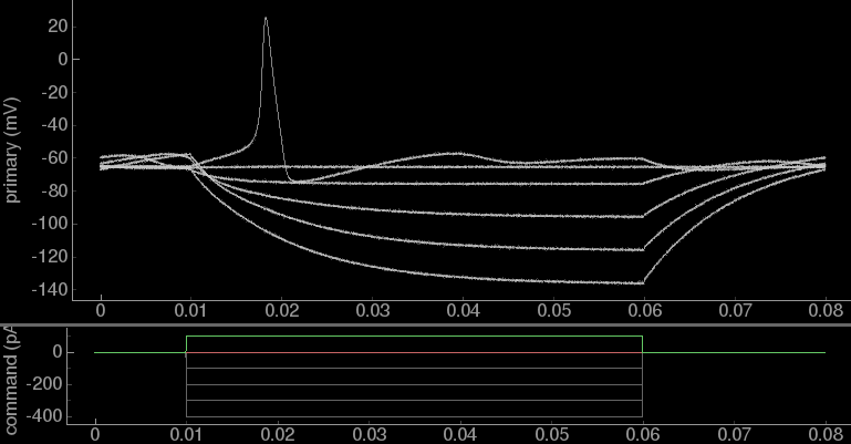
Plotting, video, and most other scientific graphics in ACQ4 are dispalyed in graphics views provided by PyQtGraph.

Mouse interaction

All graphics views in ACQ4 may be scaled and panned to interactively explore the displayed data. For this purpose it is recommended to use a standard 3-button (with wheel) mouse; however, a simplified interaction mode may be used for one-button mice (see mouse mode below). By default, graphics views have the following mouse interaction:

• Right-drag causes the view to zoom. In most cases, dragging the mouse to the right will cause the data to stretch horizontally, whereas dragging the mouse upward will cause the data to stretch vertically. However, some views have a fixed aspect ratio (such as when viewing most images); in this case dragging will always cause both axes to scale proportionally.

• Middle-drag causes the view to pan, allowing different parts of the data to be viewed.

• Left-drag is used to interact with any movable objects such as selection areas and ROIs. In the absence of such an object, left-dragging the mouse will instead pan the view exactly as middle-dragging does.

• Wheel is used to zoom the view proportionally.

In many instances, the graphics view includes x- and y-axes displayed at the edges of the view. In this case, the mouse interactions described above may be performed over either axis to limit changes to that axis. For example, rolling the mouse wheel over the y-axis causes the view to scale vertically.

View context menus

Further options are available by right-clicking to open a context menu.

• View all causes the view to zoom once such that all data is visible.

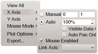
• X and Y axis menus have the following options:

  • Manual allows the range spanned by the axis to be manually fixed at the specified values.

  • Auto causes the view to automatically scale to fit any new data within the view. This is particularly useful for plots that are continuously updating with new data. The numerical value indicates the percentile of the data that will be visible, allowing automatic scaling to exclude outliers. Note that dragging the view (as described above) will cause automatic scaling to be temporarily disabled.

  • Visible data only is used when only a portion of the data is visible in the view (for example, when looking at a short section of a much longer plot). In this case, the automatic scaling only considers that part of the data which lies inside the view.

  • Auto pan only causes the auto-scaling mechanism to only re-center on the average value of the data, without rescaling. This is useful for continuously updating plots where it is desirable to be able to easily compare the amplitude of a signal as the data updates.

  • Mouse enabled specifies whether any of the mouse-dragging operations described above will affect the given axis. This is typically used to lock one axis while allowing the other to be manipulated with the mouse.

  • Invert axis indicates whether the direction of increasing value should be reversed from the default.

  • Link axis allows the ranges of two plots to be linked together such that the data they display may be compared with the same scaling and alignment.

• Mouse mode allows selection between the default 3-button mouse mode (described above) and a simplified interaction mode that is more natural for one-button mice. In this mode, a scrolling motion (typically a two-finger swipe) will zoom the plot exactly as the mouse wheel, while dragging the mouse will draw a rectangular area to be zoomed. 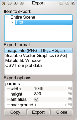This mouse mode may be configured as the default by adding defaultMouseMode: 'onebutton' to your top-level configuration file.

• Export causes an export dialog to be displayed which allows the contents of the graphics view to be exported to various file formats. For generating publication graphics, it is recommended to export to SVG, then further modify the figure with a vector graphics editor such as Inkscape or Illustrator. Alternately, CSV and HDF5 files may be exported to allow other analysis packages immediate access to the plot data.

  

Plot context menus

Graphics views that contain plot data typically include an extra Plot options context menu with features related to plotting:

• Transforms

  • FFT transforms the plot data using a fast fourier transform.

  • Log X and Y cause the plot data to be transformed logarithmically.

• Average allows multiple plots in the same graphics view to be averaged together. This is most commonly used with task runner sequences to allow repeated trials to be averaged together. In the case of multi-dimensional sequences, it is possible to select the sequence parameters which should be averaged together.

• Downsample reduces the number of samples being displayed to improve performance for large datasets. The downsampling ratio may be specified manually, or chosen automatically based on the pixel-width of the graphics view.

  

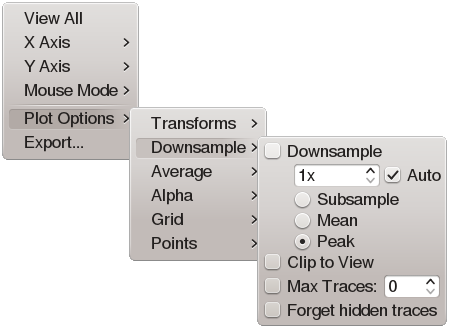
  • Three downsampling modes are available:

    • Subsample causes every Nth sample to be displayed, with all others omitted. This is the fastest option, but can lead to noisy or erratic plot display.

    • Mean causes each group of N samples to be averaged together, with a single point displayed for each. This type of downsampling reduces the apparent noise level in the displayed data.

    • Peak displays two samples for every N: the minimum and maximum values. This is the slowest option, but produces the best results when it is important to maintain the visible envelope of the signal and noise.

  • Clip to view causes any data which is not visible in the current view range to be omitted. Combined with the downsampling options above, this allows very large datasets to be displayed with good performance. It is also recommended to use both options when exporting to SVG because most vector graphics editors are not designed for use with the high-density sampled plots.

  • Max traces indicates the maximum number of plots that may be displayed at once. This is particularly useful when a large number of plots are continuously added to the graphics view; often it is desirable to plot only one or a few traces at a time.

  • Forget hidden traces is used in conjunction with max traces to remove any hidden traces permanently from memory. This is important when a large number of traces might otherwise consume an excessive amount of memory.